Ultra Fast Metropolis-Hastings Algorithm in High Dimensions

Introduction

Review of Metropolis-Hastings Algorithm

Implementing a Metropolis-Hastings Algorithm in R

Suppose we want to generate a zero-mean 2-dimensional (2D) spatial Gaussian random field from an exponential spatial covariance function model on a $50 \times 50$ grid on the unit square similar to the 2D spatial Gaussian random field in Figure 1 below.

The values in Figure 1 were generated with only a line of code using the function rmvn() in the R package mgcv. This is because generating values from the multivariate Gaussian distribution is easy and can be accomplished in a few steps. The rmvn() function performs these steps internally and returns values from the multivariate Gaussian distribution. Check out this article on how to simulate from the multivariate Gaussian distribution using dedicated functions in R.

Despite having a straightforward and convenient way to generate samples from the multivariate Gaussian distribution, the MH algorithm is also an alternative way to accomplish the required task. Doing so will also be a good exercise in showing the novelty of the MH algorithm in generating samples from a target distribution. In the following, a step-by-step implementation from scratch of the MH algorithm in R is illustrated.

1. Specify the target distribution $p(\mathbf{x})$.

   • We want to generate samples $\mathbf{Z} = \{ Z (\mathbf{s}_1), \ldots, Z (\mathbf{s}_{n}) \}^{\top} \in \mathbb{R}^{n}$ where $Z (\mathbf{s})$ is the value at spatial location $\mathbf{s} \in \mathbb{R}^{d}$. Here $n$ is the number of spatial locations and $d$ is the dimension of the spatial location. In the 50 $\times$ 50 grid example above, the value of $n$ is 2,500. For flat surfaces where spatial locations are defined by the position along the $x$ and $y$ axes, the value of $d$ is 2. The following R codes show how to generate a 50 $\times$ 50 grid:

      
     M <- 50
     n.loc <- M*M 
     locs <- cbind(rep(0:(M-1), M)/(M-1), rep(0:(M-1), each=M)/(M-1))
                                                     

     To visualize the grid, the following R codes show the x and y axes and plot the locations we constructed above.

      
     plot(locs, pch = 20, xlab = '', ylab = '')
     mtext(expression(s[x]), 1, line = 2)
     mtext(expression(s[y]), 2, line = 2)
                                                     

     The following plot should appear on the bottom-right portion of your RStudio session.

     

     The $s_x$ notation in the plot above indicates the $x$-coordinate of location. Similarly, $s_y$ indicates the $y$-coordinate.

   • We want $\mathbf{Z}$ to come from a multivariate Gaussian distribution. If $\mathbf{Z}$ is from a multivariate Gaussian distribution, we write $\mathbf{Z} \sim \mathcal{N}_{n} (\boldsymbol{\mu}, \boldsymbol{\Sigma})$, where $\boldsymbol{\mu}$ is the $n \times 1$ mean vector of $\mathbf{Z}$ and $\boldsymbol{\Sigma}$ is the $n \times n$ covariance matrix of $\mathbf{Z}$. This means that $$\text{E}(\mathbf{Z}) = [ \text{E}\{Z (\mathbf{s}_1)\}, \ldots, \text{E}\{Z (\mathbf{s}_{n})\}]^{\top} = \{ \mu (\mathbf{s}_1), \ldots, \mu (\mathbf{s}_{n}) \}^{\top} = \boldsymbol{\mu} \quad \text{ and }$$ $$\begin{bmatrix} \text{cov}\{Z (\mathbf{s}_1), Z (\mathbf{s}_1)\} & \text{cov}\{Z (\mathbf{s}_1), Z (\mathbf{s}_2)\} & \cdots & \text{cov}\{Z (\mathbf{s}_1), Z (\mathbf{s}_n)\} \\ \text{cov}\{Z (\mathbf{s}_2), Z (\mathbf{s}_1)\} & \text{cov}\{Z (\mathbf{s}_2), Z (\mathbf{s}_2)\} & \cdots & \text{cov}\{Z (\mathbf{s}_2), Z (\mathbf{s}_n)\} \\ \vdots & \vdots & \ddots & \vdots \\ \text{cov}\{Z (\mathbf{s}_n), Z (\mathbf{s}_1)\} & \text{cov}\{Z (\mathbf{s}_n), Z (\mathbf{s}_2)\} & \cdots & \text{cov}\{Z (\mathbf{s}_n), Z (\mathbf{s}_n)\} \end{bmatrix} = \begin{bmatrix} \Sigma_{11} & \Sigma_{12} & \cdots & \Sigma_{1n} \\ \Sigma_{21} & \Sigma_{22} & \cdots & \Sigma_{2n} \\ \vdots & \vdots & \ddots & \vdots \\ \Sigma_{n1} & \Sigma_{n2} & \cdots & \Sigma_{nn} \\ \end{bmatrix} = \boldsymbol{\Sigma}.$$

   1. Code the mean of the target distribution.

      We want $\mathbf{Z}$ to be zero-mean, meaning we set $\boldsymbol{\mu}$ to be the zero vector. In R, this can be done as follows:

      
      mu <- rep(0, n.loc)
      	                                        

      The R variable mu above is a vector consisting of 2,500 zeros. Printing the values of mu on the R console will look like this:

      

   2. Code the covariance of the target distribution.

      We want the covariances between the components of $\mathbf{Z}$, namely, $Z (\mathbf{s}_1), Z (\mathbf{s}_2), \ldots, Z (\mathbf{s}_n)$, to be modeled by the exponential spatial covariance function. This means that $$\text{cov}\{Z (\mathbf{s}_i), Z (\mathbf{s}_j)\} = \sigma^2 \exp \left( -\frac{\|\mathbf{s}_i - \mathbf{s}_j \|}{a} \right),$$ where $\sigma^2$ and $a$ are the nonnegative parameters of the exponential spatial covariance function. Here, $\sigma^2$ is the variance parameter, while $a$ is the spatial range parameter. You can set the values of these parameters to any nonnegative value. However, note that the parameter values will control the statistical properties of the $\mathbf{Z}$ that will be generated later on. The following R codes set the parameter values equal to the ones used to generate the $\mathbf{Z}$ values in Figure 1.

      
      sigma2 = 1
      a = 0.5
      	                                        

      The symbol $\| \cdot \|$ indicates that we need to solve for the Euclidean distance between locations $\mathbf{s}_i$ and $\mathbf{s}_j$. Remember that the Euclidean distance can be computed using the formula: $$ \|\mathbf{s}_i - \mathbf{s}_j \| = \sqrt{(s_{i1} - s_{j1})^2 + (s_{i2} - s_{j2})^2 + \ldots + (s_{id} - s_{jd})^2}.$$ When $d = 2$, meaning we only have the $x$ and $y$ axes to describe the location, the Euclidean distance formula simplifies to: $$ \|\mathbf{s}_i - \mathbf{s}_j \| = \sqrt{(s_{ix} - s_{jx})^2 + (s_{iy} - s_{jy})^2}.$$ Given a matrix of locations such as locs, the distance between any two locations can be computed systematically using the R function dist(). This can be done as follows:

      
      dist_matrix <- as.matrix(dist(locs))
      	                                        

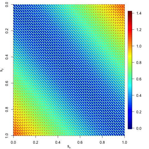
      Note that dist_matrix is a 2,500 $\times$ 2,500 matrix of distances, where the $i$th and $j$th entry of the matrix is the Euclidean distance between locations $\mathbf{s}_i$ and $\mathbf{s}_j$. We can visualize the distances by plotting an image of the dist_matrix using the image.plot() function in the R package fields. The following codes detail how this can be done in R:

       
      install.packages("fields")
      library(fields)
      image.plot(dist_matrix, ylim=c(max(locs[, 2]),0))
      mtext(expression(s[x]), 1, line = 2)
      mtext(expression(s[y]), 2, line = 2)
                                                      

      The following plot should appear on the bottom-right portion of your RStudio session.

      

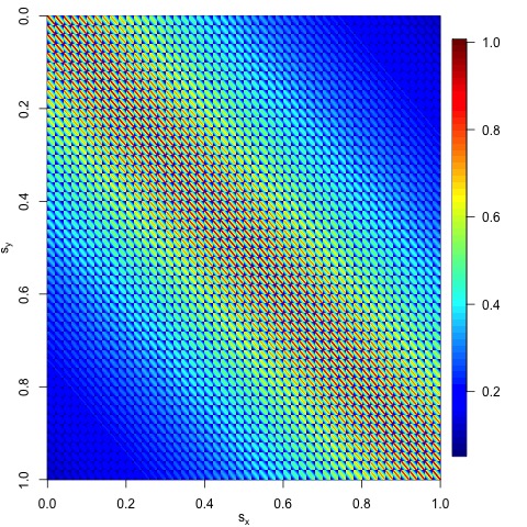
      Now that we have the parameter values and the distances, we can now compute the values of the entries inside the covariance matrix $\boldsymbol{\Sigma}$. The covariance matrix can easily be computed with one line of R code as follows:

       
      cov_matrix <- sigma2 * exp(-dist_matrix/ a)
                                                      

      The code above simply executes the formula for the exponential covariance function. Note that cov_matrix is a 2,500 $\times$ 2,500 matrix of covariances, where the $i$th and $j$th entry of the matrix is the value of the exponential covariance function evaluated with locations $\mathbf{s}_i$ and $\mathbf{s}_j$. We can visualize $\boldsymbol{\Sigma}$ by plotting an image of the cov_matrix as follows:

       
      image.plot(cov_matrix, ylim=c(max(locs[, 2]),0))
      mtext(expression(s[x]), 1, line = 2)
      mtext(expression(s[y]), 2, line = 2)
                                                      

      The following plot should appear on the bottom-right portion of your RStudio session.

      

   3. Code the function that will compute the density of the target distribution.

      Given the mean vector mu and the covariance matrix cov_matrix, we can now code a function that will compute the density of our target distribution. The multivariate Gaussian density has the form: $$p(\mathbf{z} | \boldsymbol{\mu}, \boldsymbol{\Sigma}) = \frac{1}{(2 \pi)^{n/2} |\boldsymbol{\Sigma}|^{1/2}} \exp \left\{ -\frac{1}{2} (\mathbf{z} - \boldsymbol{\mu})^{\top}\boldsymbol{\Sigma}^{-1} (\mathbf{z} - \boldsymbol{\mu})\right\}, $$ where $\mathbf{z}$ is any vector in $\mathbb{R}^n$.

      In practice, we often work with the logarithmic transformation of the multivariate Gaussian density. This makes it easier for computers to store and handle very small probability values. The multivariate Gaussian log density has the form: $$\ln \{ p(\mathbf{z} | \boldsymbol{\mu}, \boldsymbol{\Sigma})\} = -\frac{n}{2} \log(2 \pi) - \frac{1}{2} \log (|\boldsymbol{\Sigma}|) -\frac{1}{2} (\mathbf{z} - \boldsymbol{\mu})^{\top}\boldsymbol{\Sigma}^{-1} (\mathbf{z} - \boldsymbol{\mu}). $$ The following codes define a function that will compute the target log density. When performing the MH algorithm, we can disregard the other components of the multivariate Gaussian log density that do not depend on $\mathbf{z}$ as shown in the R function below.

       
      target_log_density <- function(z, mu, sigma_inv){
        return(-0.5*(t(z-mu) %*% sigma_inv %*% (z-mu)))
      }
                                              

2. Specify the proposal (conditional) distribution $q(\mathbf{z}^{\text{new}} | \mathbf{z}^{\text{old}})$.

   Here, $\mathbf{z}^{\text{old}}$ denotes the last accepted sample in the chain and $\mathbf{z}^{\text{new}}$ is the newly proposed (not yet accepted or rejected) sample.

   There are two most commonly used types of proposal distributions, namely, (a) independent and (b) random-walk.

   1. Independent proposal distributions are those that do not depend on $\mathbf{z}^{\text{old}}$, the most current accepted sample in the chain. This means that $$q(\mathbf{z}^{\text{new}} | \mathbf{z}^{\text{old}}) = q(\mathbf{z}^{\text{new}}).$$ For instance, $$q(\mathbf{z}^{\text{new}}) = \mathcal{N}_{n} (\mathbf{z}^{\text{new}} | \boldsymbol{\mu}, \boldsymbol{\Sigma}).$$ This approach is ideal when the proposal distribution is known to approximate well the target distribution.
   2. Proposal distributions under the random walk approach are those that depend on the value from the previous iteration, $\mathbf{z}^{\text{old}}$. Moreover, the proposal distribution will be centered around $\mathbf{z}^{\text{old}}$. For example, if the proposal distribution is the following: $$q(\mathbf{z}^{\text{new}} | \mathbf{z}^{\text{old}}) = \mathcal{N}_{n}(\mathbf{z}^{\text{new}} | \mathbf{z}^{\text{old}}, \boldsymbol{\Sigma}),$$ then this means that the proposal distribution is the multivariate Gaussian distribution with mean $\mathbf{z}^{\text{old}}$ and covariance matrix $\boldsymbol{\Sigma}$. Note that the random walk proposal distribution above is symmetric since $$\mathcal{N}_{n}(\mathbf{z}^{\text{new}} | \mathbf{z}^{\text{old}}, \boldsymbol{\Sigma}) = \frac{1}{(2 \pi)^{n/2} |\boldsymbol{\Sigma}|^{1/2}} \exp \left\{ -\frac{1}{2} (\mathbf{z}^{\text{new}} - \mathbf{z}^{\text{old}})^{\top}\boldsymbol{\Sigma}^{-1} (\mathbf{z}^{\text{new}} - \mathbf{z}^{\text{old}})\right\} $$ is equal to $$\mathcal{N}_{n}(\mathbf{z}^{\text{old}} | \mathbf{z}^{\text{new}}, \boldsymbol{\Sigma}) = \frac{1}{(2 \pi)^{n/2} |\boldsymbol{\Sigma}|^{1/2}} \exp \left\{ -\frac{1}{2} (\mathbf{z}^{\text{old}} - \mathbf{z}^{\text{new}})^{\top}\boldsymbol{\Sigma}^{-1} (\mathbf{z}^{\text{old}} - \mathbf{z}^{\text{new}})\right\}.$$ This means that $q(\mathbf{z}^{\text{new}} | \mathbf{z}^{\text{old}}) = q(\mathbf{z}^{\text{old}} | \mathbf{z}^{\text{new}})$.
3. Code the MH algorithm.
   1. Initialize the chain with an arbitrary value for $\mathbf{z}_0$. For example, $\mathbf{z}_0$ can be the zero vector.

       
      z0 <- rep(0, n.loc)
                                                      

   2. Set the value of $\mathbf{z}_{\text{old}}$ to $\mathbf{z}_0$.

       
      z.old <- z0
                                                      

   3. Set the number of iterations that the MH algorithm will perform.

       
      n.epoch <- 10000
                                                      

   4. Define a matrix where we can store the values of the current vector at every iteration.

       
      out <- matrix(NA, nrow=length(mu), ncol=n.epoch + 1)
                                                      

   5. For $r = 1, \ldots,$n.epoch, repeat the following steps:
      1. Generate $\mathbf{z}_{\text{new}}$, a candidate vector to be the next vector in the chain, from the proposal distribution.

          
         eps <- 0.1
         z.new <- z + runif(length(mu), -eps, eps)
                                                                 

      2. Calculate the acceptance probability $A$. Since we are working with log densities, we can translate the acceptance ratio above to its equivalent log acceptance ratio. $$\log A = \min \left[0, \log \{p(\mathbf{z}_{\text{new}})\} - \log \{p(\mathbf{z}_{\text{old}})\} \right].$$

          
         Sigma_inv <- solve(Sigma)
         p.new <- target_log_density(z.new, mu, Sigma_inv)
         p.old <- target_log_density(z.old, mu, Sigma_inv)
         log.A <- min(p.new - p.old, 0)
                                                                 

      3. Generate $u$ from the uniform distribution $U[0, 1]$.

          
         u <- runif(n=1, min=0, max=1)
                                                                 

      4. Accept $\mathbf{z}_{\text{new}}$ as the next vector in the chain if $u \leq \alpha$. Otherwise, do not update the value of $\mathbf{z}_{\text{old}}$.

          
         if(log(u) <= log.A){
           z.old <- z.new
         }
                                                                 

      5. Store the values of the current vector in the chain.

          
         out[,r+1] <- z.old
                                                                 

Problems of Metropolis-Hastings Algorithm in High Dimensions

Principle Behind the Metropolis-Adjusted Langevin Algorithm